Bernstein-Vazirani algorithm (Part 2): How to run your algorithms on a realistic quantum computer
In the last part of the previous series, Deutsch algorithm, I introduced a manual way to construct the oracle. That oracle must be built from matrix because the oracle function is undeterminate except for the outcome. In Bernsterin-Vazirani problem, the function is, on the other hand, clearly stated: $f(\mathbf{x}) = \mathbf{s}\cdot\mathbf{x}$. So, it’s unnecessary to repeat the previous procedure; instead, we’ll build the oracle without using matrices by understanding what the function really do. There are two slightly different way to build the oracle, and we’ll also execute the whole algorithms on both simulators and IBM’s quantum computers.
Python & Qiskit
From now on, I’ll switch to write demo code using Python and Qiskit, a well-designed Python-based library for quantum computing. The library also supports the use of realized quantum computers developed by IBM so that you can execute your algorithm within your computer simulator or by requesting IBM to do that for you.
There is a great “Getting Started” for the library. You can pip install the library and follow the instruction above to get familiar with its syntax. It’s not difficult at all. Another suggestion is that you should look for basic tutorials in Qiskit Github as well.
Then we're gonna come straight into the implementation: Given a bitstring $\mathbf{s}$, we need to initialize our computation with at least $n$ qubits, where $n$ is the length of $\mathbf{s}$, plus $1$ ancilla qubit for phase kickback.
| |
Next we'll create the backbone of the circuit:
| |
A set of gates for preparation is also applied at the beginning. It is very common to use this subroutine in a variety of quantum algorithms
| |
Oracle construction
Recalling that $U_f|x\rangle|y\rangle = |x\rangle|y\oplus f(x)\rangle$ is no other than a NOT gate acting on $|y\rangle$ controlled by the value of $f(x)$. Therefore, we need to come up with a way to find out every $\mathbf{x}$ that $f(\mathbf{x})=1$, which is equivalent to $\mathbf{s}\cdot\mathbf{x}=1$. The dot product $s_1s_2...s_n \cdot x_1x_2...x_n$ can only be equal $1$ when $s_i = x_i = 1$ for an odd number of $i$ indexes. All the three other types of $s_i,x_i$ pair do not contribute to the product result. So, what we need to do is to apply $CNOT |x_i\rangle|y\rangle$ where $s_i = 1$. It's easily to see that the operator is a NOT gate acting on the ancilla when $s_i= x_i = 1$. Moreover, the value $y$ will experience a net change only if the NOT gate is applied an odd number of times. Sounds a little bit complicated? See the code to figure it out.
| |
Finish it up
The last gates are applied to retrieve the bitstring as well as get the circuit returned to a standard state. Here I draw out the circuit with “latex” backend. If you haven’t installed LaTeX locally, you can either use “mpl” for matplotlib backend or default “text” backend.
| |
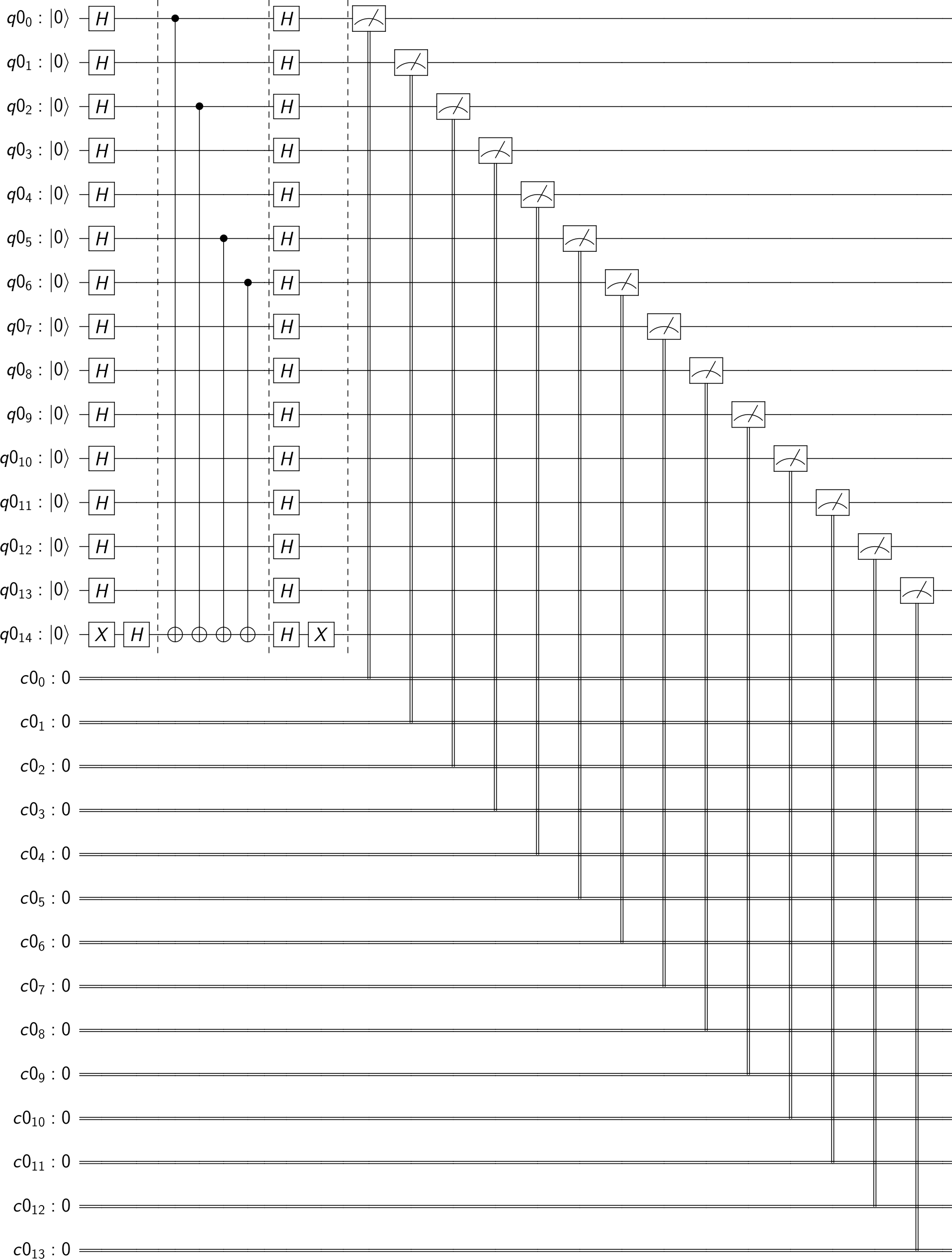
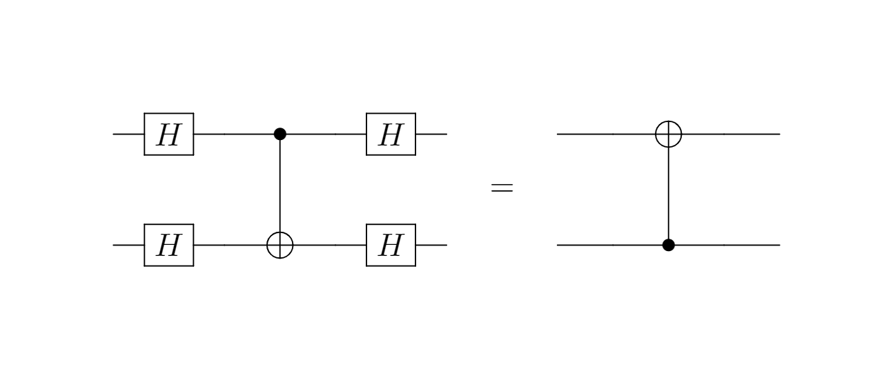
I’ll analyze the circuit a little bit further. Mathematically, it’s not so difficult to prove the equality $(\mathbf{H}_0\otimes\mathbf{H}_1) \mathbf{CNOT}_{0,1} (\mathbf{H}_0\otimes\mathbf{H}_1) = \mathbf{CNOT}_{1,0}$
Squeezing the ancilla between two $X$ gates, we get
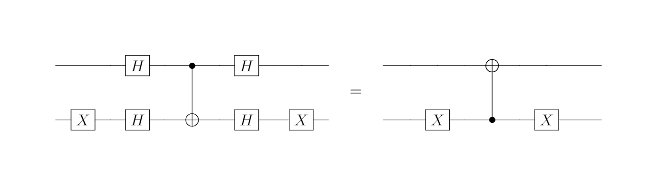
The figure above obviously points out that every qubit that has a CNOT connnection with the ancilla will be changed to the state $|1\rangle$ at the end of the circuit. The positions of changed qubits corresponds to the positions of the string $s$ whose bits are $1$. This is absolutely what we want.
Executing the algorithm on different calculating backends
Once finish implementing, you can run the algorithm in two different ways. The first one is using your local simulator, which utilizes the computing power of your CPU. This is certainly not the target of quantum computing, but it’s really convenient that you can check your algorithm accuracy for a small number of qubits. The second way is borrowing computing power of quantum devices available for public use from large players in the field (IBM, Rigetti to name a few). Unfortunately, because we still rest at an era called Noisy-Intermediate Scale Quantum (NISQ), so you shouldn’t expect much from the performance of those public quantum computers.
The two chunks of code below show the difference in implementations and results betweeb using a simulator and a IBM’s quantum computer.
| |
| |
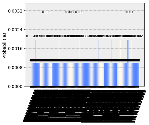
You see the result… The correct result not even shows up once out of $1024$ times (You can check dictionary “answer” on your own). Merely outputing random strings, it can’t be any worse. The main reason for this phenomenon comes from the fact CNOT gates belong to the set of multiqubit operators and are difficult to engineered precisely. Still, there are tons of technical barriers we must confront ahead. However, there is a brighter, instant way for us to improve our computation performance: A circuit without multiqubit gates definitely results in a better outcome. That’s what I want to introduce in the next section.
Alternative circuit design
Before diving into a new circuit design for the algorithm, you should keep in mind that THE LESS CONTROL GATES THE CIRCUIT HAS, THE MORE PRECISE ITS OUTCOME CAN BE. So, our purpose is to create an circuit with all gates being single-qubit.
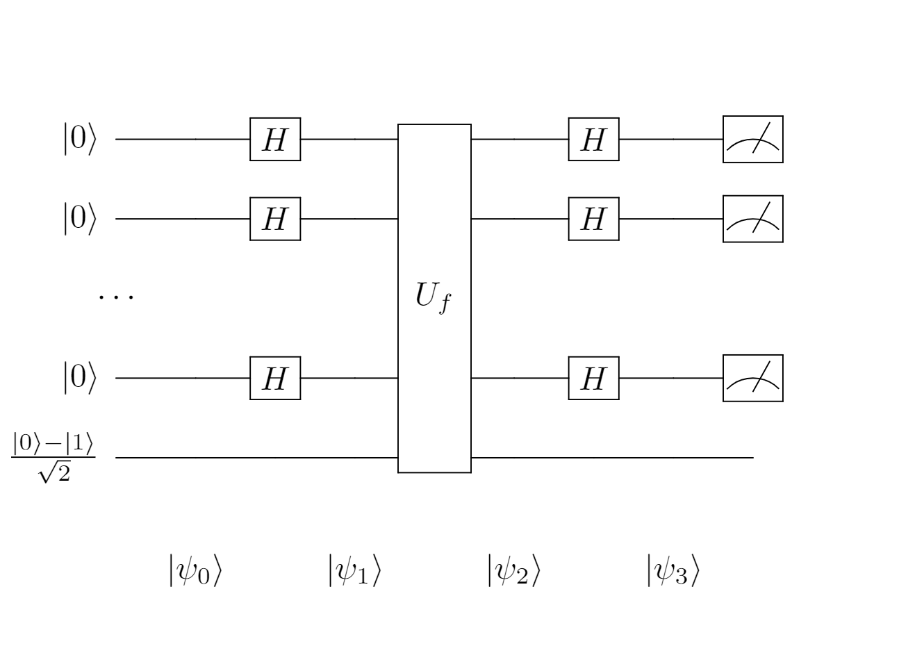 In terms of the circuit above, looking back all the states $|\psi\rangle$ calculated in Part 2, we notice that the ancilla qubit is always kept in the state $\frac{|0\rangle - |1\rangle}{\sqrt{2}}$:
$$|\psi_0\rangle = |0\rangle^{\otimes n} \left( \frac{|0\rangle - |1\rangle}{\sqrt{2}}\right)$$
$$|\psi_1\rangle = \frac{1}{\sqrt{2^n}}\sum_{\mathbf{x} \in \{0,1\}^n} |\mathbf{x}\rangle \left( \frac{|0\rangle - |1\rangle}{\sqrt{2}}\right)$$
$$|\psi_2\rangle = \frac{1}{\sqrt{2^n}} \sum_{\mathbf{x} \in \{0,1\}^n} (-1)^{\mathbf{s}\cdot\mathbf{x}} |\mathbf{x}\rangle \left( \frac{|0\rangle - |1\rangle}{\sqrt{2}} \right)$$
$$|\psi_3\rangle = \frac{1}{\sqrt{2^n}} \sum_{\mathbf{z} \in \{0,1\}^n} (-1)^{\mathbf{s}\cdot\mathbf{x} \oplus \mathbf{x}\cdot\mathbf{z}} |\mathbf{z}\rangle \left( \frac{|0\rangle - |1\rangle}{\sqrt{2}} \right)$$
In terms of the circuit above, looking back all the states $|\psi\rangle$ calculated in Part 2, we notice that the ancilla qubit is always kept in the state $\frac{|0\rangle - |1\rangle}{\sqrt{2}}$:
$$|\psi_0\rangle = |0\rangle^{\otimes n} \left( \frac{|0\rangle - |1\rangle}{\sqrt{2}}\right)$$
$$|\psi_1\rangle = \frac{1}{\sqrt{2^n}}\sum_{\mathbf{x} \in \{0,1\}^n} |\mathbf{x}\rangle \left( \frac{|0\rangle - |1\rangle}{\sqrt{2}}\right)$$
$$|\psi_2\rangle = \frac{1}{\sqrt{2^n}} \sum_{\mathbf{x} \in \{0,1\}^n} (-1)^{\mathbf{s}\cdot\mathbf{x}} |\mathbf{x}\rangle \left( \frac{|0\rangle - |1\rangle}{\sqrt{2}} \right)$$
$$|\psi_3\rangle = \frac{1}{\sqrt{2^n}} \sum_{\mathbf{z} \in \{0,1\}^n} (-1)^{\mathbf{s}\cdot\mathbf{x} \oplus \mathbf{x}\cdot\mathbf{z}} |\mathbf{z}\rangle \left( \frac{|0\rangle - |1\rangle}{\sqrt{2}} \right)$$
If the ancilla stays constant throughout calculation, is it really meaningful? Is it possible to eliminate the ancilla from our equation? The answer turns out to be yes. In fact, the ancilla serves the only purpose of phase kick-back whose effect can be summerized in one equation: $$U_f: |x\rangle \left( \frac{|0\rangle - |1\rangle}{\sqrt{2}} \right) \mapsto (-1)^{f(x)} |x\rangle \left( \frac{|0\rangle - |1\rangle}{\sqrt{2}} \right)$$ As long as we can produce $(-1)^{f(x)} |x\rangle$, it’s no point to keep the ancilla. A single-qubit operator that is able to reverse the sign with regard to the value of $f(x)$ is Z gate. Having the matrix form of $\begin{bmatrix} 1 & 0\\ 0 & -1 \end{bmatrix}$, it keeps the state $|0\rangle$ unchanged and transforms $|1\rangle$ into $-|1\rangle$. We can redo the same procedure in the sections above: finding out every $\mathbf{x}$ that $f(\mathbf{x})=1$ and apply the Z gate to those positions. The code doesn’t change much:
| |
Initializing and running the circuit on the realized quantum device used the original circuit:
| |
| |
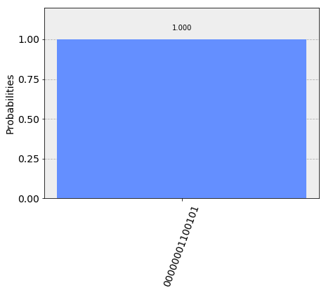
Here’s the result
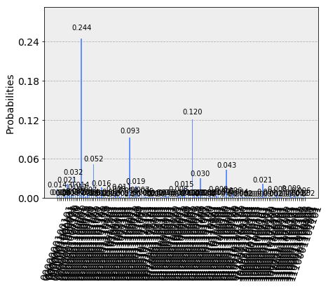 The code chunk below is for extracting the correct value of $\mathbf{s}$, which is the bitstring of highest possibility in the chart.
| |
Although the chart still shows a tremedously errorneous result, at least the correct outcome stays distinguishable from other wrong outcomes. From all the examples in this article, I hope you got a basic understanding of Qiskit and real quantum computers. Quantumly performing an algorithm is a way to help figure out what can be done and what is yet to be done in the quantum realm. Again, feel free to explore my code stored in my GitHub repository.
My little suggestion: Take a look at Transpiler, a special class for quantum hardware optimization.