Randomized Benchmarking (Part 2): Protocols for standard and interleaved versions + Experiment with a realistic quantum device

Knowing the underpinnings of randomized benchmarking addressed in the last part, we first begin with the standard protocol. Standard RB is used to assess the error rate over gates of Clifford group with an assumption that these gates have the same error rate. After that, another improvement of the technique will be introduced, namely Interleaved Randomized Benchmarking. The upgraded version was proposed not to investigate the Clifford group as a whole, but restricted to one single kind of Clifford gate of our choice. In this text, we’re going to figure out how to do randomized benchmarking as well as what’s the difference between the two versions’ protocols and derived models.

Standard Randomized Benchmarking Protocol

First, the Clifford group of gates is denoted as Cliff. For a chosen Cliff, the RB protocol is decribed as follows:

1. Choose a sequence length $m \in \mathbb{N}$.
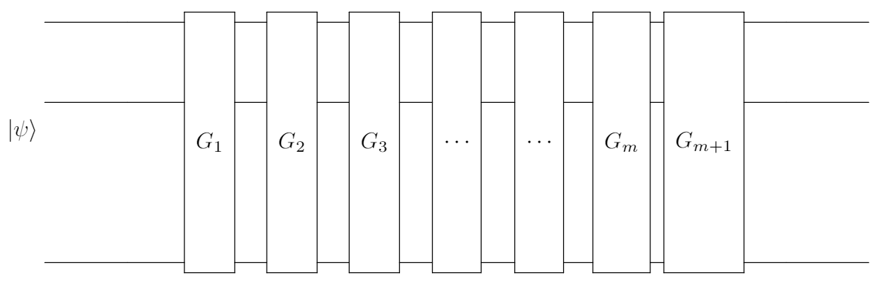
2. Sample a sequence of $m$ gates $(G_1,G_2,…,G_m)$ with $G_i$ being picked independently and uniformly randomly from Cliff.
3. Prepare an initial state $\rho \approx |0\rangle\langle 0|$ in the current $d$-dimensional system. Here $\rho$ is a quantum state that takes into account state-preparation errors experimentally.
4. Determine the inversion operator of the sampled sequence from step 2 $G_{m+1} = \left(\bigcirc_{i=1}^{m}G_i \right)^{-1}$. If the sampled sequence was composed of Clifford operates, it is assured that the inversion will also be in the Clifford group.
5. Apply the new sequence $\mathcal{G} = G_{m+1} \circ G_{m} \circ … \circ G_{1}$.
6. Measure a POVM $\{E, I-E\}$, where the first element $E$, which takes into account measurement errors, associates to the survival possibility of the initial state at the end of the sequence.
7. Repeat step 3 – 6 a number of times to estimate the probability that the initial state is not changed by the sequence, Pr(“survival”|$E$,$m$) = $\text{Tr} \left[ E\mathcal{G}\left(\rho\right)\right]$. The survival probability will be $1$ for every sequence in the ideal (noiseless) circumstance.
8. Repeat step 2 – 7 for $K$ different sequences. The average survival probability over the $K$ sequences represents the sequence fidelity $F_{\text{avg}}(m)$.
9. Repeat step 1 – 8 for various choices of $m$ and fit the results to the exponential decay model: $$F(m) = A_{\mathcal{E}}p^m + B_{\mathcal{E}}$$

Two parameters $A_{\mathcal{E}}$ and $B_{\mathcal{E}}$ absorb state-preparation, measurement errors and the error occuring at the final gate $G_{m+1}$ within the channel of gate-independent error $\mathcal{E}$. The models outputs the depolarizing parameter $p$. Recalling 2 equations from part 1, $$p = \frac{dF_{\text{avg}}-1}{d-1} \text{ and } r = 1 - F_{\text{avg}},$$ the average infidelity (also average error rate in this case) over Clifford group is given by $r = \frac{(d-1)(1-p)}{d}$, where $d=2^n$ is the dimension of the system. In the case of 1-qubit randomized benchmarking, the formula for evaluating average error rate is reduced to $r = \frac{1-p}{2}$.

Interleaved Randomized Benchmarking Protocol

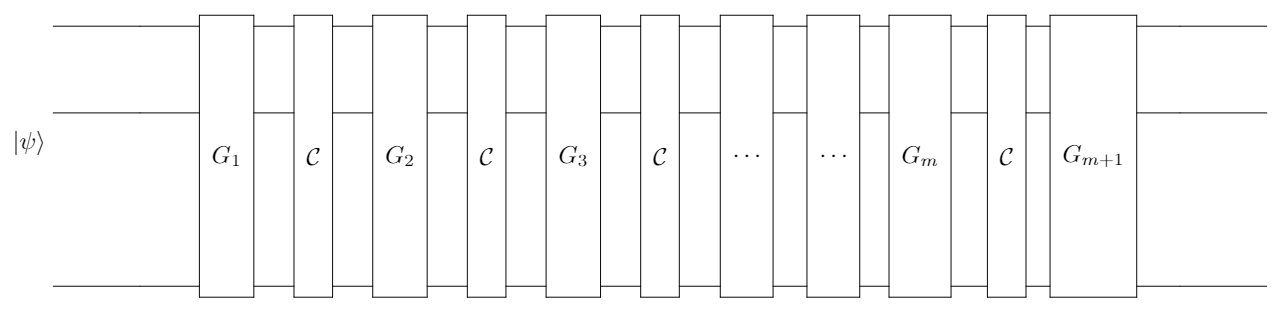
In comparison with the standard version, the protocol for interleaved randomized benchmarking doesn’t change much, except that for every operator $G_i$ for ($1 \leq i \leq m$), a designated operator $\mathcal{C} \in$ Cliff will be laid aside. $\mathcal{C}$ is the specific gate of which we want to determine the error rate. This version is named interleaved RB also for putting $\mathcal{C}$ between every pairs of $G_i$. However, we still keep the convention of defining the sequence length by the number of random gates.

The final gate is the inverse of $m$ pairs of $G_i$ and $\mathcal{C}$ for every $1 \leq i \leq m$: $$G_{m+1} = \left(\bigcirc_{i=1}^{m}\left(\mathcal{C} \circ G_i\right) \right)^{-1}$$ The operator that represents the whole sequence now becomes $$\mathcal{G} = G_{m+1} \circ \mathcal{C} \circ G_{m} \circ … \circ \mathcal{C} \circ G_{1}$$

Other steps in the protocol remains unchanged. The decay model results in a different depolarizing parameter $p_{\mathcal{C}}$. Acknowledging the standard depolarizing paratemter $p$, the error rate of the target gate can be estimated by $$\bar{r}_{\mathcal{C}} = \frac{(d-1)(1-\frac{p_{\mathcal{C}}}{p})}{d},$$ and must lie in the range $\left[\bar{r}_{\mathcal{C}} +\sigma,\bar{r}_{\mathcal{C}} -\sigma \right]$, where

$$\sigma = \text{min} \left\{\begin{matrix} \frac{(d-1)\left[ \left| p - \frac{p_{\mathcal{C}}}{p} \right| + (1-p) \right ]}{d} \\
\frac{2\left(d^2-1\right)\left(1-p\right)}{pd^2} + \frac{4\sqrt{1-p}\sqrt{d^2-1}}{p} \end{matrix}\right.$$

Implementation

I have written some Python code to perform both versions of RB, examining 14 qubits of “ibmq_16_melbourne” quantum device built by IBM. Please note that we’re only considering sing-qubit benchmarking so that operators applied on each qubit are working independently, thus $d = 2^1 = 2$ for every benchmarking. I initialize the experiment using the following function:

 1
 2
 3
 4
 5
 6
 7
 8
 9
10
11
12
13
14
15
16
17
18
19
20
21
22

def circuit_generator():
    #Number of seeds (random sequences)
    nseeds = 5
    
    #Number of Cliffords in the sequence (start, stop, steps)
    nCliffs = np.arange(1,200,20)
    
    rb_pattern = [[0],[1],[2],[3],[4],[5],[6],[7],[8],[9],[10],[11],[12],[13]]
    
    length_multiplier = 1

    interleaved_gates = [['h 0'], ['h 0'], ['h 0'], ['h 0'], ['h 0'], ['h 0'], ['h 0'], ['h 0'], ['h 0'], ['h 0'], ['h 0'], ['h 0'], ['h 0'], ['h 0']]
    
    rb_opts = {}
    rb_opts['length_vector'] = nCliffs
    rb_opts['nseeds'] = nseeds
    rb_opts['rb_pattern'] = rb_pattern
    rb_opts['length_multiplier'] = length_multiplier
    rb_opts['interleaved_gates'] = interleaved_gates
    rb_original_circs, xdata, rb_interleaved_circs = rb.randomized_benchmarking_seq(**rb_opts)

    return rb_original_circs, rb_interleaved_circs, xdata, rb_opts 

In comparison with the theory, nseeds is $K$, the number of repetition for each value $m$, nCliffs = [1,21,41,61,81,101,121,141,161,181] is the set of various value of $m$ (in this case, we do RB with 10 $m$’s). The variable rb_pattern describes that there are 14 independent and concurrent single-qubit benchmarkings on qubits indexed 0 to 13. The interleaved gate chosen here is Hadamard gate appied in the 0th qubit of the corresponding benchmarking. The helper function rb.randomized_benchmarking_seq(**rb_opts) creates all necessary sequences for standard and interleaved RB stored in rb_original_circs and rb_interleaved_circs respectively.

After the sequences get executed with the mentioned backend, the results are ready for the fitting curve model. Fortunately, Qiskit already has great support for this part.

1
2
3
4
5
6

#Create the original and interleaved RB fitter
original_rb_fit = rb.RBFitter(original_result_list, xdata, rb_opts['rb_pattern'])
interleaved_rb_fit = rb.RBFitter(interleaved_result_list, xdata, rb_opts['rb_pattern'])

#Calculate the joint fitter
joint_rb_fit = rb.InterleavedRBFitter(original_result_list, interleaved_result_list, xdata, rb_opts['rb_pattern']) 

The last thing is to draw out figures corresponding to the benchmarked qubits based on the resulting fitters.

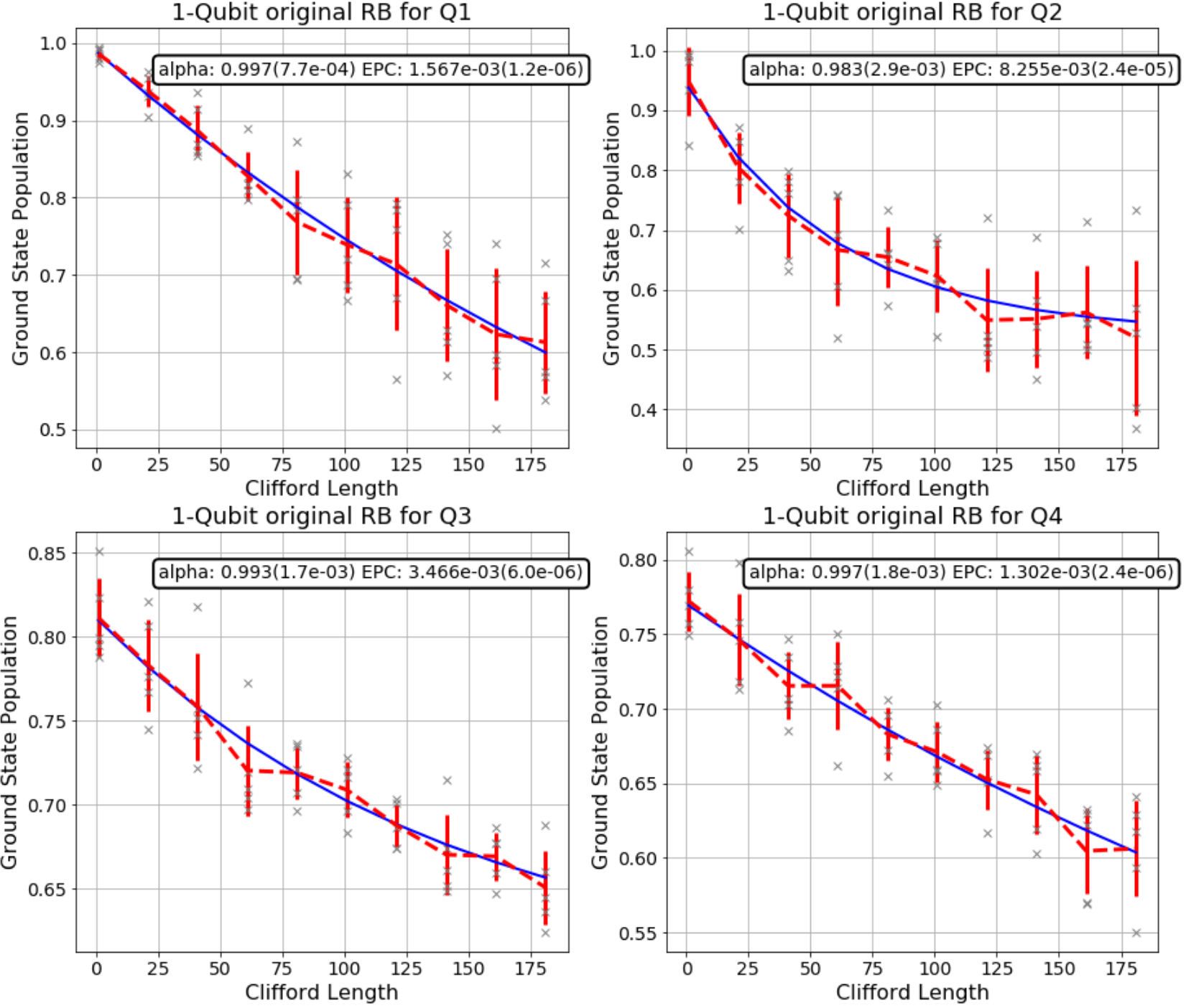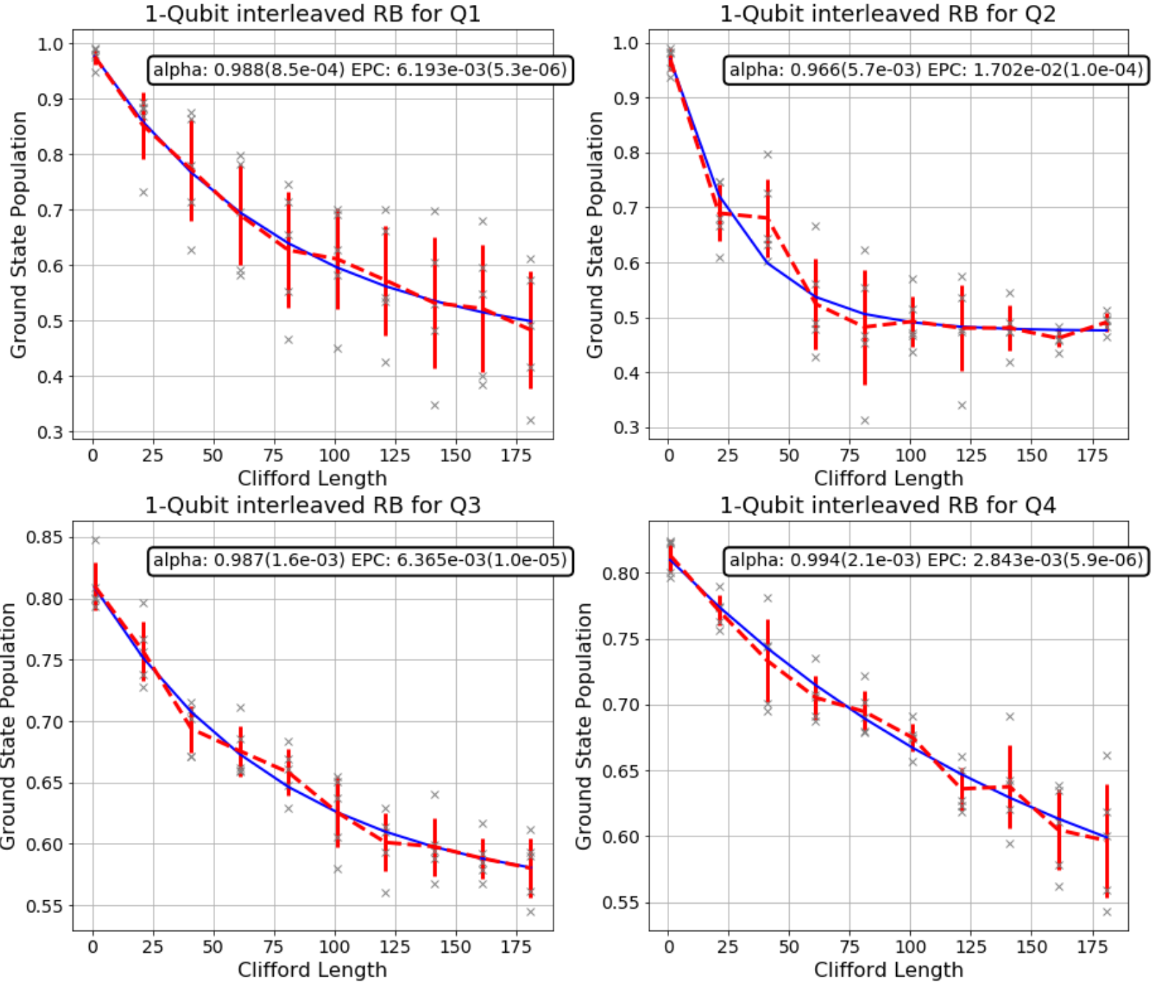Merging these two graphs highlights that the Hadamard gates in the IBMQ device we used seems to not have good quality compared to the average of Clifford gates.

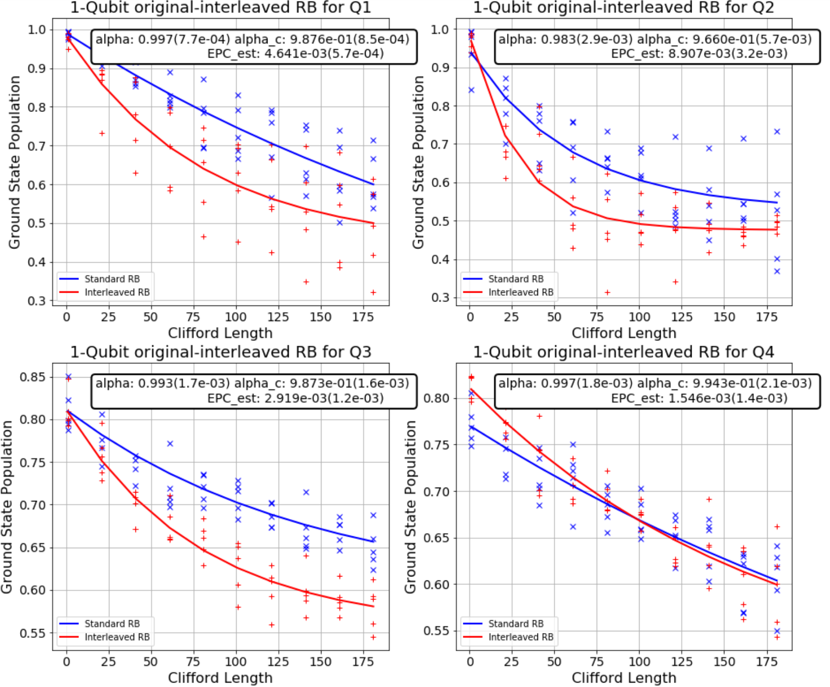
(If you have seen my Python notebook, you might notice that I am only successful in benchmarking the first 4 qubits. All the other ones show unexpected result that I have no idea what is going on. My mentor said that IBM may restrict the number of gates applied to the 10 remaining qubits and suggesting me to run the algorithm for each batch of 4 qubits. But I’m too lazy for this, it really took a lot of time to run :<)

Before we come to the end, I’ll show you the fidelity, which in this case means the rate at which a gate transforms the quantum state correctly, of Clifford group in general and of Hadamard gate, both corresponding to each out of 4 successfully benchmarked qubits.

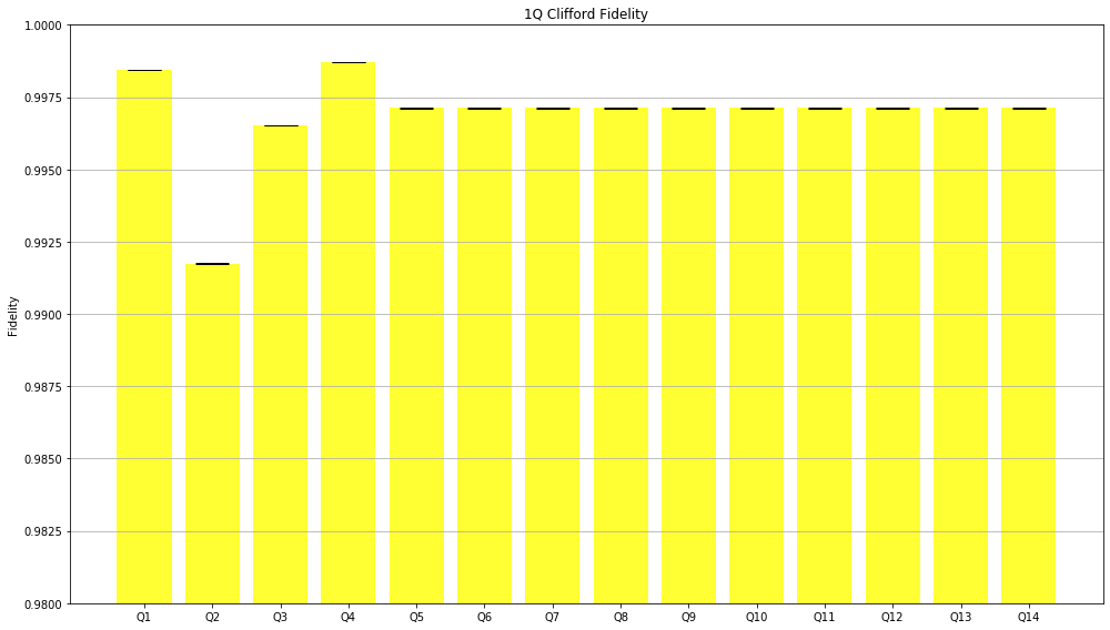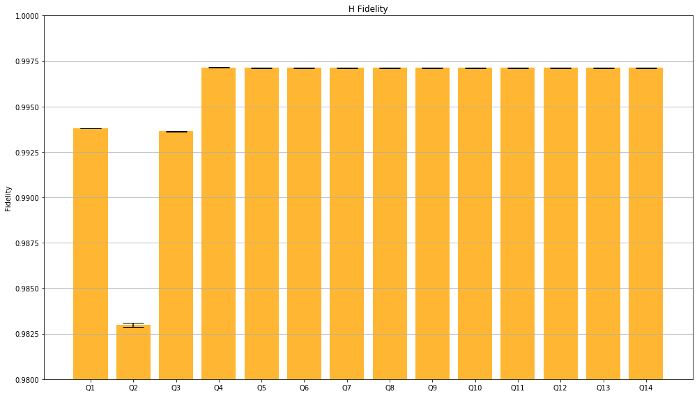Probably IBM needs to do something with the second qubit…

Here is my code (the interleaved notebook would be more sufficient) in case you desire to benchmark any IBM’s qubit and gate. Have fun!