Introduction

In this NISQ (Noisy Intermediate Scale Quantum) era, scientists hold much expectation for three applications of Quantum Computing: Quantum Fourier Transform-based algorithms, Grover-search-based algorithms, and simulations of quantum phenomena (as in Quantum Chemistry). In this series, we want to discuss Shor’s algorithm, the most prominent instance of the first type. Shor’s original work attracted huge attention since it showed a strong evidence that 2048-bit RSA, a widely used cryptographic protocol in the Internet communication, can be broken (Technology is switching to post-quantum cryptography though). The protocol relies on a belief that it is hard to factor large number into two large prime numbers $N=pq$ (but unsure if it is NP-hard). Shor proposed an efficient quantum algorithm for the factorization, making heavy use of Quantum Fourier Transform (QFT) and Quantum Phase Estimation (QPE). These two have widespread application as subroutines of a huge spectrum of quantum algorithms. QFT and QPE are even seen as of much more practical importance than the Shor’s algorithm itself. For that reason, this document will mainly cover QFT and leave QPE and Shor’s algorithm for later posts.

Fourier Transform

Fourier Transform has been known for its importance in signal processing. It decomposes a signal, or a time function, into $\sin$ and $\cos$ constituents. The transformation allows changing between the signal’s time domain and frequency domain as the following illustration¹.

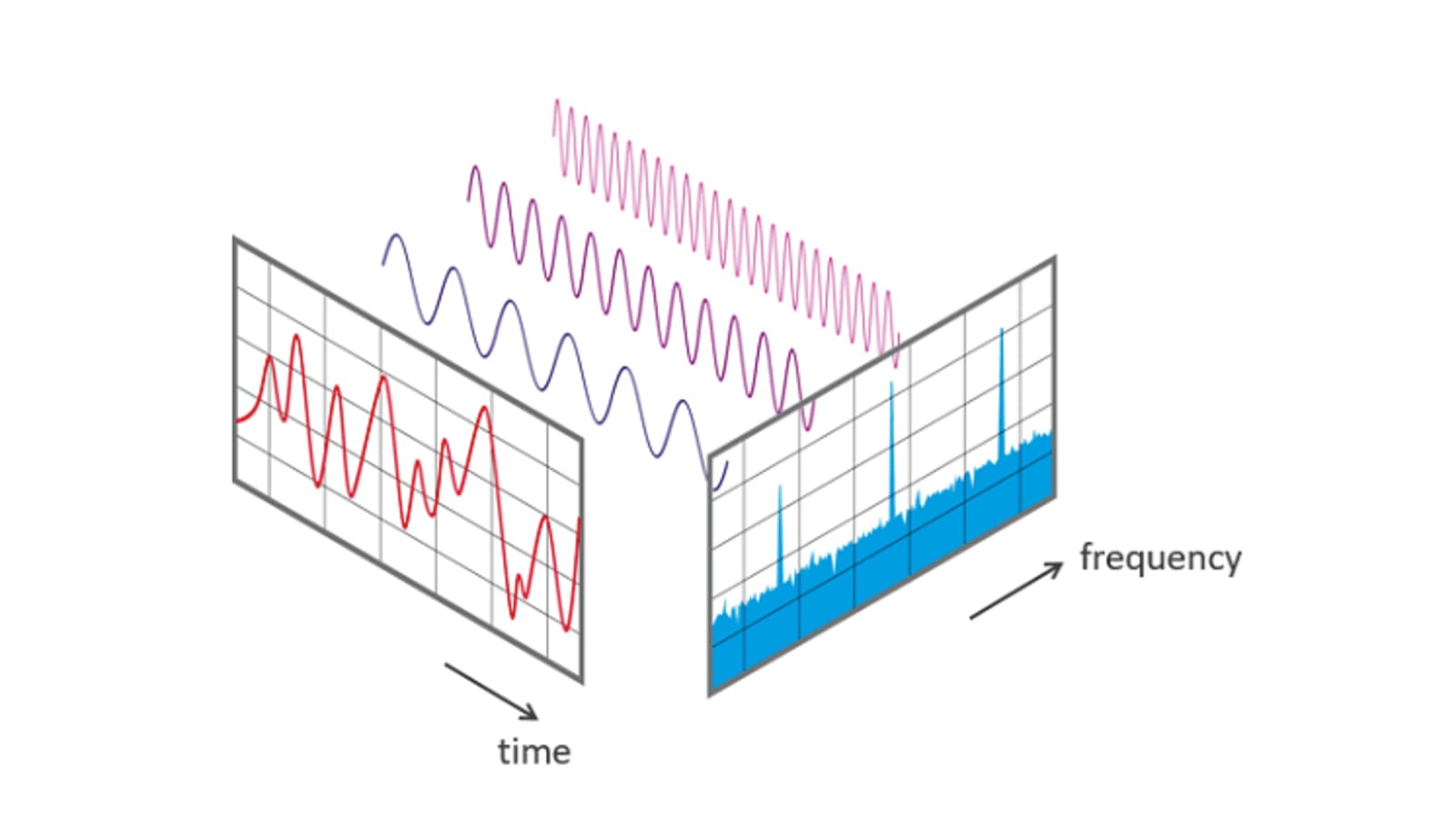
The transform analyzes and casts light on the periodicity of the given signal, which later proves to be helpful to the whole problem of factorization. Mathematically, the (discrete) Fourier transform takes $x=\begin{bmatrix}x_0 \\ x_1 \\ \vdots \\ x_{N-1} \end{bmatrix} \in \mathbb{C}^N$ as input and returns $y=\begin{bmatrix}y_0\\ y_1 \\ \vdots \\ y_{N-1} \end{bmatrix} \in \mathbb{C}^{N}$, where $$y_k = \frac{1}{\sqrt{N}} \sum_{j=0}^{N-1} x_je^{2\pi ijk/N}$$

For more information, 3Blue1Brown made a nice illustrative video lecture about Fourier Transform and how it maps time/spatial domain to frequency domain.

Quantum Fourier Transform

Definition and Examples

The QFT is exactly the same, except for little notational change. It performs a change of basis from the computational basis $|0\rangle, |1\rangle, \dots, |N-1\rangle$ to the Fourier basis $$|\tilde{x}\rangle \equiv QFT|x\rangle = \frac{1}{\sqrt{N}}\sum_{y=0}^{N-1} e^{2\pi ixy/N} |y\rangle$$

QFT, as a quantum operator, needs to be unitary. Show that $QFT QFT^{\dagger} = QFT^{\dagger}QFT = I$, given $QFT^{\dagger}|x\rangle = \frac{1}{\sqrt{N}}\sum_{y=0}^{N-1} e^{-2\pi ixy/N} |y\rangle$, and therefore QFT is a unitary operator.

For example, $N=2^1 = 2$ for 1 qubit, $$\begin{matrix} QFT|x\rangle &=& \frac{1}{\sqrt{2}}\sum_{y=0}^{N-1} e^{2\pi ixy/N} |y\rangle \\ &=& \frac{1}{\sqrt{2}} \left[e^{2\pi ix\cdot 0/2}|0\rangle + e^{2\pi ix\cdot 1{/}2}|1\rangle\right] \\
&=& \frac{1}{\sqrt{2}} \left[|0\rangle + e^{\pi ix}|1\rangle\right] \end{matrix}$$ $$QFT|0\rangle = \frac{1}{\sqrt{2}} \left[|0\rangle + e^{\pi i\cdot 0}|1\rangle\right] = \frac{1}{\sqrt{2}} \left(|0\rangle + |1\rangle\right) =|+\rangle$$ $$QFT|1\rangle = \frac{1}{\sqrt{2}} \left[|0\rangle + e^{\pi i\cdot 1}|1\rangle\right] = \frac{1}{\sqrt{2}} \left(|0\rangle - |1\rangle\right) =|-\rangle$$

The notations of $|3\rangle, |4\rangle,\dots$, in fact, make use of multiple qubits as a string of binary numbers. As a matter of fact, $|4\rangle$ is $|100\rangle$ or $|0100\rangle$ corresponding to a system composed of 3 or 4 qubits respectively. The summation of kets can also be viewed as taking sum across every qubit in the system $$\sum_{y=0}^n|y\rangle \rightarrow \sum_{y_1=0}^1 \sum_{y_2=0}^1 \dots \sum_{y_n=0}^1 |y_1y_2\dots y_n\rangle $$

For a general system of $n$ qubits, the maximum number of possible states is $N=2^n$. Viewed as a bitstring, $y = [y_1y_2\dots y_n] = 2^{n-1}y_1 + 2^{n-2}y_2 + \dots + 2^{0}y_n = \sum_{k=1}^n y_{k}2^{n-k}$, which implies $\frac {y}{N} = \sum_{k=1}^n \frac{y_{k}}{2^k}$.

Equivalently, the action of the QFT on the composite state can be pinned down to separate qubits

$$\displaystyle{\begin{matrix} |\tilde{x}\rangle &=& \frac{1}{\sqrt{N}}\sum_{y=0}^{N-1} e^{2\pi ixy/N} |y\rangle \\
&=& \frac{1}{\sqrt{N}}\sum_{y=0}^{N-1} e^{2\pi ix \sum_{k=1}^n y_k/2^k} \\
&=& \frac{1}{\sqrt{N}}\sum_{y=0}^{N-1} \prod_{k=1}^n e^{\frac{2\pi ixy_k}{2^k}} |y_1 y_2 \dots y_n\rangle \\
&=& \frac{1}{\sqrt{N}}\sum_{y_1=0}^{1} \sum_{y_2=0}^{1} \dots \sum_{y_n=0}^{1} \prod_{k=1}^n e^{\frac{2\pi ixy_k}{2^k}} |y_1 y_2 \dots y_n\rangle \\
&=& \frac{1}{\sqrt{N}} \left(|0\rangle + e^{\frac{2\pi ix}{2^1}}|1\rangle\right) \otimes \left(|0\rangle + e^{\frac{2\pi ix}{2^2}}|1\rangle\right) \otimes \dots \otimes \left(|0\rangle + e^{\frac{2\pi ix}{2^n}}|1\rangle\right) \end{matrix}}$$

The QFT maps $|x\rangle = |x_1\rangle \otimes |x_2\rangle \otimes \dots \otimes |x_n\rangle$ to $\frac{1}{\sqrt{N}} \left(|0\rangle + e^{\frac{2\pi ix}{2^1}}|1\rangle\right) \otimes \left(|0\rangle + e^{\frac{2\pi ix}{2^2}}|1\rangle\right) \otimes \dots \otimes \left(|0\rangle + e^{\frac{2\pi ix}{2^n}}|1\rangle\right) $. Qubit-wise, it maps $|x_k\rangle$ to $\frac{1}{\sqrt{2}}\left(e^{\frac{2\pi ix\cdot 0}{2^k}}|0\rangle + e^{\frac{2\pi ix\cdot 1}{2^k}}|1\rangle\right) = \frac{1}{\sqrt{2}}\left(|0\rangle + e^{\frac{2\pi ix}{2^k}}|1\rangle\right)$.

For example, $|x\rangle = |4\rangle = |100\rangle$. From the representation $N = 2^3 = 8$

$$QFT|x\rangle = |\tilde{x}\rangle = |\tilde{4}\rangle = \frac{1}{\sqrt{8}}\left(|0\rangle + e^{\frac{2\pi i\cdot 4}{2}}|1\rangle \right) \otimes \left(|0\rangle + e^{\frac{2\pi i\cdot 4}{4}}|1\rangle \right) \otimes \left(|0\rangle + e^{\frac{2\pi i\cdot 4}{8}}|1\rangle \right)$$

Construction of circuit

Ingredients

Because QFT maps $|x_k\rangle$ to $|\tilde{x}_k\rangle = \frac{1}{\sqrt{2}}\left(|0\rangle + e^{\frac{2\pi ix}{2^k}}|1\rangle\right)$, the post-QFT state is a superposition of all the states in the Hilbert space of the system. The coefficients in the superposition are $|00\dots 00\rangle, e^{2\pi ix/2^n}|00\dots 01\rangle$, $e^{2\pi ix/2^{n-1}}|00\dots 10\rangle$, $e^{2\pi ix\left(\frac{1}{2^n}+\frac{1}{2^{n-1}}\right)}|00\dots 11\rangle$ up to $e^{2\pi ix\left(\frac{1}{2}+\frac{1}{2^2}+\dots+\frac{1}{2^n}\right)}|11\dots 11\rangle$. To express in words, (1) the phase of each qubit is dependent to both $n$ qubits, and (2) the more “1”’s in a term, the more terms present in the sum in the relative phase $e^{2\pi ix(… + …)}$.

This observation hints the form of the circuit. Before introducing the circuit, we first take a look at two essential types of one-qubit gates that will occur on it.

The first gate is simply the Hadamard gate. Recalling that $H|0\rangle = \frac{1}{\sqrt{2}} \left(|0\rangle + |1\rangle \right)$ and $H|1\rangle = \frac{1}{\sqrt{2}} \left(|0\rangle - |1\rangle \right)$, the gate’s action can be written compactly as $H|x_j\rangle = \frac{1}{\sqrt{2}}\left(|0\rangle + e^{\frac{2\pi i x_j}{2}}|1\rangle\right)$.

The second gate, named $R_k$, maps $|x_j\rangle$ to $e^{\frac{2\pi i x_j}{2^k}|x_j\rangle}$. From the definition, $R_k|0\rangle = e^{\frac{2\pi i \cdot 0}{2^k}}|0\rangle = |0\rangle$ and $R_k|1\rangle = e^{\frac{2\pi i}{2^k}}|1\rangle$. The gate $R_k$ can be written in matrix as $$R_k = \begin{bmatrix} 1 & 0 \\
0 & e^{\frac{2\pi i}{2^k}} \end{bmatrix}$$ The action of this gate is to change the relative phase, equivalent to a one-qubit rotation about the Z axis that can be implemented with the U1 gate in qiskit. Nonetheless, we need to be able to apply this gate depending on the state of other qubits. Then we choose the simplest version of a controlled gate, $CR_k$ that acts on one control qubit and one target qubit. In the following expression, assume the control qubit to be the first one. $$\begin{matrix} CR_k &=& |0\rangle\langle 0|\otimes I + |1\rangle \langle 1| \otimes R_k \\
&=& \begin{bmatrix} 1 & 0 & 0 & 0 \\
0 & 1 & 0 & 0 \\
0 & 0 & 1 & 0 \\
0 & 0 & 0 & e^{2\pi i/2^k} \end{bmatrix} \end{matrix}$$

For completeness, you can verify that $CR_k = CNOT \cdot \left(I \otimes R_{k+1} \right)^{\dagger} \cdot CNOT \cdot \left(R_{k+1} \otimes I \right) \cdot \left(I \otimes R_{k+1} \right)$. This decomposition shows a sequence of one-qubit rotation gate along with CNOT is equivalent to the controlled-rotation gate. In general, any $d \times d$ unitary gate can be decomposed into a sequence of single qubit rotation and CNOT. That allows a convenient comparison between the number of operations needed for a computation between classical devices and quantum devices.

Circuit model

The circuit is as follow.

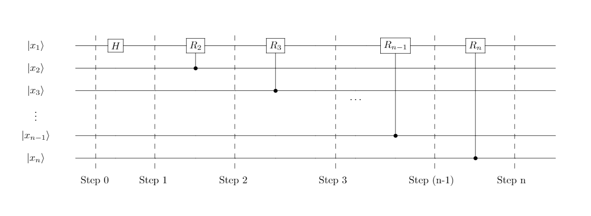
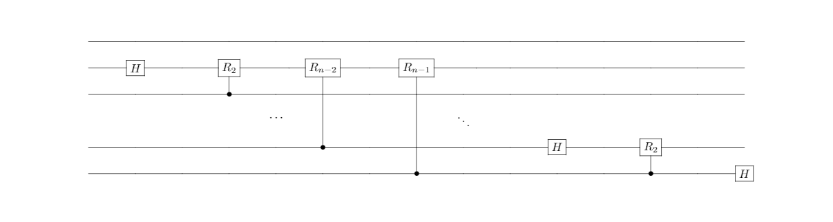
As you can see, each qubit, as the target, effectively experiences the operator $\dots CR_3 CR_2 H$. We show that this circuit produces the same effect as of $QFT$, except that the last outcome is reversed. This means that reversing the order of the qubits at the end yields the desired outcome. For illustration, we attempt to write out all transformations related to the first qubit, ie. up to Step n. $$ \begin{matrix} \text{Step 0:} & |x_1x_2\dots x_n\rangle \\
\text{Step 1:} & \frac{1}{\sqrt{2}} \left(|0\rangle + e^{\frac{2\pi i}{2^1}x_1} |1\rangle\right) |x_2x_3\dots x_n\rangle \\
\text{Step 2:} & \frac{1}{\sqrt{2}} \left(|0\rangle + e^{\frac{2\pi i}{2^2}x_2}e^{\frac{2\pi i}{2^1}x_1} |1\rangle \right) |x_2x_3\dots x_n\rangle \\
\text{Step 3:} & \frac{1}{\sqrt{2}} \left(|0\rangle + e^{\frac{2\pi i}{2^3}x_3}e^{\frac{2\pi i}{2^2}x_2}e^{\frac{2\pi i}{2^1}x_1} |1\rangle\right) |x_2x_3\dots x_n\rangle \\
\text{Step n:} & \frac{1}{\sqrt{2}} \left(|0\rangle + e^{\frac{2\pi i}{2^n}x_n} \dots e^{\frac{2\pi i}{2^3}x_3}e^{\frac{2\pi i}{2^2}x_2}e^{\frac{2\pi i}{2^1}x_1} |1\rangle\right) |x_2x_3\dots x_n\rangle \\
& = \frac{1}{\sqrt{2}} \left( |0\rangle + e^{\frac{2\pi i}{2^n}x}|1\rangle\right)|x_2x_3\dots x_n\rangle \end{matrix}$$ The last equation comes from the identity $\frac{x}{2^m} = \frac{x_n}{2^m} + \frac{x_{n-1}}{2^{m-1}} + \dots + \frac{x_{n-m+1}}{2^{1}}$ One can attempt to compute the transformation of the other qubits, with a note that $e^{2\pi i \cdot z} = 1 \text{ for } z\in \mathbb{N}$, and arrive at the final state $$ \frac{1}{\sqrt{2^n}} \left( |0\rangle + e^{\frac{2\pi i}{2^n}x}|1\rangle\right) \otimes \left( |0\rangle + e^{\frac{2\pi i}{2^{n-1}}x}|1\rangle\right) \otimes \dots \otimes \left( |0\rangle + e^{\frac{2\pi i}{2^1}x}|1\rangle\right)$$ This state is indeed $|\tilde{x}\rangle$ yet in reversed order. If necessary, one can apply $SWAP$ on the qubits pair by pair to retain $|\tilde{x}\rangle$.

Recall that for a unitary $U = U_1U_2\dots U_n$, $U^{\dagger} = U^{\dagger}_n\dots U^{\dagger}_2 U^{\dagger}_1$. One can express the circuit for $QFT$ in this form and then find the circuit for $QFT^{\dagger}$.

Advantage of QFT over classical Fourier Transform

In this section we compare the efficiency of QFT and DFT (Discrete Fourier Transform) by counting the number of elementary operations used for the two paradigms.

Naively thinking, $N$ complex multiplication and $N$ addition suffice for a computation of $y_k = \frac{1}{\sqrt{N}} \sum_{j=0}^{N-1} x_je^{2\pi ijk/N}$. Since there are $N$ terms $y_k$, so naive DFT takes $O(N^2) = O(2^{2n}) = O(2^n)$ operations.

In reality, Fast Fourier Transform (FFT) is in more favor. The improvement relies on several symmetries of the coefficients of $y_k$ and effectively reduces the complexity to $O(N\log{N}) = O(n2^n)$. For more information, this note presents DFT and FFT in depth.

On the other hand, QFT only needs $n$ gates for the first qubit, $n-1$ gates for the second qubit, and so on, that sum up to $n+(n-1)+\dots +1 = n(n+1)/2$. Even if we take into account n/2 $SWAP$ gates (each can be implemented by 3 $CNOT$ gates) and the decomposition of $CR_k$ into single-qubit rotations and $CNOT$ gates, the quantum circuit still only needs $O(n^2)$ operations. Exponential speedup! The problem, as in any other quantum algorithm, is that there is no physical way to extract the coefficients right away from the superposition without destroying it. As a result, any algorithm that uses QFT as a subroutine, should be designed to subtly leverage the superposition without a direct measurement.

References

[1] Quantum Computation and Quantum Information (Chapter 5), Nielsen & Chuang
[2] CS191 Lecture Note from EdX UC Berkeley.
[3] IBM qiskit textbook (you’ll find a good instruction for implementation there)